By Hans Kurzweil
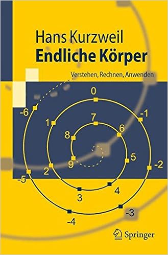
In jedem convenient, CD-Player und desktop steckt ein Chip, der lineare Gleichungssystem über einem endlichen Körper blitzschnell löst, um fehlerbehaftetes Datenmaterial zu korrigieren; dieses Buch erklärt additionally das mathematische Innenleben eines solchen Chips. Endliche Körper (sogenannte Galoisfelder) sind Zahlbereiche mit nur endlich vielen Zahlen, die guy trotzdem addieren, subtrahieren, multiplizieren und dividieren kann. Das Hauptanliegen des Buches ist es, auf elementare Weise zu erklären und zu üben, wie diese Rechnungen ausgeführt werden. In der Praxis beruht diese Arithmetik auf der 0,1- Arithmetik des pcs. Ein endlicher Körper mit 2 Elementen besteht aus den bits 0,1; acht bits erklären ein byte, und diese bytes sind die Elemente eines Körpers mit 256 Elementen.
Das Buch wendet sich an jeden, dem die mathematischen Sprache nicht fremd ist und der wissen möchte, wie endliche Körper funktionieren. Vorausgesetzt wird eine gewisse Vertrautheit mit den Grundbegriffen der linearen Algebra, wie sie etwa in einer Vorlesung Ingenieurmathematik geübt werden. Obwohl der textual content zielgerichtet ist, bietet er auch eine elementare Einführung in die Algebra, denn endliche Körper können ohne die Begriffe - Gruppe, Vektorraum, Ring, Körper und Polynom - nicht erklärt werden.
Read Online or Download Endliche Korper: Verstehen, Rechnen, Anwenden PDF
Similar discrete mathematics books
Computational Complexity of Sequential and Parallel Algorithms
This e-book offers a compact but entire survey of significant ends up in the computational complexity of sequential algorithms. this can be by way of a hugely informative creation to the advance of parallel algorithms, with the emphasis on non-numerical algorithms. the fabric is so chosen that the reader in lots of situations is ready to keep on with an identical challenge for which either sequential and parallel algorithms are mentioned - the simultaneous presentation of sequential and parallel algorithms for fixing permitting the reader to recognize their universal and targeted gains.
Discontinuum Mechanics : Using Finite and Discrete Elements
Textbook introducing the mathematical and computational thoughts of touch mechanics that are used more and more in business and educational software of the mixed finite/discrete aspect strategy.
Matroids: A Geometric Introduction
Matroid concept is a colourful region of analysis that gives a unified method to comprehend graph idea, linear algebra and combinatorics through finite geometry. This e-book presents the 1st complete advent to the sector with a view to entice undergraduate scholars and to any mathematician drawn to the geometric method of matroids.
Fragile networks: Identifying Vulnerabilities and Synergies in an Uncertain World
A unified therapy of the vulnerabilities that exist in real-world community systems-with instruments to spot synergies for mergers and acquisitions Fragile Networks: choosing Vulnerabilities and Synergies in an doubtful global provides a complete examine of community structures and the jobs those platforms play in our daily lives.
Additional info for Endliche Korper: Verstehen, Rechnen, Anwenden
Sample text
Grad λA = grad A, wenn λ = 0. 2. grad (A + B) ≤ max {grad A, grad B}. Dabei gilt die Gleichheit, wenn entweder grad A = grad B oder grad A = grad B und an = −bn . 3. grad A · B = grad A + grad B, wenn A = 0 = B. 1 ¨ Ofters wird in diesem Fall auch grad A = −∞ gesetzt. 22 2. Der Polynomring Der Leser mache sich diese anhand von Beispielen klar. Wir verwenden diese wichtigen Gradregeln im Folgenden meistens ohne besonderen Hinweis. Nach Definition gilt: A = 0 ⇔ grad A ≥ 0 . Deswegen folgt aus der dritten Gradregel, dass der Ring F[X] nullteilerfrei ist.
Insbesondere ist nun x das Polynom X und xi das Polynom X i , wenn i < n. 7, so folgt xn = −(d0 + d1 x + · · · + dn−1 xn−1 ) . 11 Proposition Sei N = d0 + d1 X + · · · + dn−1 X n−1 + X n . a) Der Ring FN ist auch F-Vektorraum und 1, x, . . , xn−1 ist eine Basis dieses Vektorraums. Elemente a, b ∈ FN haben daher die Form: a = a0 + a1 x + a2 x2 + · · · + an−1 xn−1 , 2 b = b0 + b1 x + b2 x + · · · + bn−1 x n−1 , ai ∈ F bi ∈ F b) a + b = (a0 + b0 ) + (a1 + b1 )x + · · · + (an−1 + bn−1 )xn−1 c) ab = ci xi , mit ci = a0 bi + a1 bi−1 + · · · + ai−1 b1 + ai b0 i d) xn = −(d0 + d1 x + .
A B Also ist F ein Skalar und V = K. Seien A, B teilerfremd. Dann ist kgV(A, B) = A · B. Beweis Das Polynom V = A · B ist gemeinsames Vielfaches von A, B. 2. 4 Lemma Das Polynom N sei ein Teiler des Produkts A · B. Sind die Polynome A und N teilerfremd, so ist N Teiler von B. Beweis A · B sowie A · N sind gemeinsame Vielfache von A und N . 3). 1 folgt A · B = F · kgV(A, N ) = F · A · N . K¨ urzt man durch A, so ist B = F · N , wie behauptet. 4 ein irreduzibles Polynom, liegt es also in P(A · B), aber nicht in P(A), so ist N ∈ P(B).